DGL 모듈을 활용한 그래프 생성
https://docs.dgl.ai/guide_ko/graph-graphs-nodes-edges.html
📖 그래프 기본적인 정의
- 에지의 방향성에 따라서, directed / undirected로 구분
- 가중치의 여부에 따라서, weighted / unweighted로 구분
- 노드의 타입이 모두 같은지 여부에 따라서 동종(homogeneous) / 이종(heterogeneous)로 구분
- 이분 그래프(bipartite graph)는 이종 그래프의 특별한 형태로, 에지는 서로 다른 두 타입의 노드를 연결. 추천 시스템에서 주로 사용됨.
✅그래프 생성하기
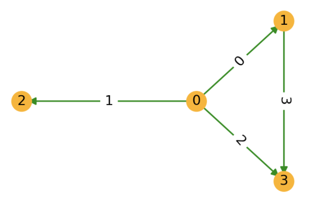
여러 노드를 표현하기 위해서 DGL는 노드 ID로 1차원 정수 텐서를 사용한다. (PyTorch의 tensor, TensorFlow의 Tensor, 또는 MXNet의 ndarry) DGL은 이 포멧을 “노드-텐서”라고 부른다. DGL에서 에지들은 노드-텐서의 튜플 (U,V) 로 표현된다. (U[i],V[i])는 U[i] 에서 V[i]로의 에지이다.
import dgl
import torch as th

# edges 0->1, 0->2, 0->3, 1->3
u, v = th.tensor([0, 0, 0, 1]), th.tensor([1, 2, 3, 3])
g = dgl.graph((u, v))

print(g)
print(g.nodes())
print(g.edges())
print(g.edges(form='all'))

# Graph(num_nodes=6, num_edges=4,
#      ndata_schemes={}
#      edata_schemes={})
#tensor([0, 1, 2, 3, 4, 5])
#(tensor([0, 0, 1, 5]), tensor([1, 2, 2, 0]))
#(tensor([0, 0, 1, 5]), tensor([1, 2, 2, 0]), tensor([0, 1, 2, 3]))
✅ 노드 및 에지의 feature 설정하기
g.ndata['feat'] = th.randn(g.num_nodes(), 5)
weights = th.tensor([0.1, 0.6, 0.9, 0.7])
g.edata['w'] = weights

print(g.ndata['feat'])
print(g.edata['w'])
#tensor([[ 0.0616,  1.6565,  0.1940, -0.5374, -0.6856],
#        [-1.7733, -1.1384,  1.3491, -0.4095, -2.8695],
#        [ 0.2854,  1.3816, -1.1483, -0.1895, -1.3160],
#        [-0.3102, -0.1107,  0.1282, -0.4775,  0.6557],
#        [-0.3523, -0.3775, -1.3288,  0.1205, -0.2521],
#        [-0.3051,  0.9397,  0.5969,  0.5036, -1.9567]])
#tensor([0.1000, 0.6000, 0.9000, 0.7000])
✅ 외부 소스를 사용한 그래프 생성하기
📖 SciPy 희소 행렬
“Scientific Python”의 줄임말로, 과학 및 공학 계산을 위한 파이썬 라이브러리이다.
scipy.sparse모듈을 통해 다양한 유형의 희소 행렬을 제공한다. 일반적인 행렬 표현(밀집 행렬, Dense Matrix)로는 메모리 사용량이 비효율적이므로, non-zero 값만 저장하여 효율성을 극대화한 데이터 구조다.
import scipy.sparse as sp

spmat = sp.rand(100, 100, density=0.05) # 5% nonzero entries
sp_graph = dgl.from_scipy(spmat)
print(sp_graph)
#Graph(num_nodes=100, num_edges=500,
#      ndata_schemes={}
#      edata_schemes={})
✅ 이종 그래프 생성하기
graph_data = {
  ('drug', 'interacts', 'drug') : (th.tensor([0, 1]), th.tensor([1, 2])),
  ('drug', 'interacts', 'gene'): (th.tensor([0, 1]), th.tensor([2, 3])),
  ('drug', 'treats', 'disease'): (th.tensor([1]), th.tensor([2]))
}

hetero = dgl.heterograph(graph_data)

print(hetero)
#Graph(num_nodes={'disease': 3, 'drug': 3, 'gene': 4},
#      num_edges={('drug', 'interacts', 'drug'): 2,
#                 ('drug', 'interacts', 'gene'): 2,
#                 ('drug', 'treats', 'disease'): 1},
#      metagraph=[('drug', 'drug', 'interacts'),
#                 ('drug', 'gene', 'interacts'),
#                 ('drug', 'disease', 'treats')])
print(hetero.ntypes)
#['disease', 'drug', 'gene']
print(hetero.etypes)
#['interacts', 'interacts', 'treats']
print(hetero.canonical_etypes)
#[('drug', 'interacts', 'drug'),
# ('drug', 'interacts', 'gene'),
# ('drug', 'treats', 'disease')]

# A homogeneous graph
# dgl.heterograph({('node_type', 'edge_type', 'node_type'): (u, v)})
# A bipartite graph
# dgl.heterograph({('source_type', 'edge_type', 'destination_type'): (u, v)})
- metagraph는 그래프의 스키마로, 노드 타입 간에 에지가 존재함을 알려준다.
# Set/get feature 'hv' for nodes of type 'drug'
hetero.nodes['drug'].data['hv'] = th.ones(3, 1)
print(hetero.nodes['drug'].data['hv'])
#tensor([[1.],
#        [1.],
#        [1.]])
# Set/get feature 'he' for edge of type 'treats'
hetero.edges['treats'].data['he'] = th.zeros(1, 1)
print(hetero.edges['treats'].data['he'])
#tensor([[0.]])
- 위와 같이 특정 노드나 에지 타입에 대한 feature를 설정할 수 있다.
✅ GPU에서 DGLGraph 사용하기
print(g.device)
#cpu
u, v = u.to('cuda:0'), v.to('cuda:0')
g = dgl.graph((u, v))
print(g.device)
#cuda:0
cuda_g = g.to('cuda:0')
print(cuda_g.device)
#cuda:0
- to() api를 사용해서 그래프 구조와 피처 데이터를 함께 gpu로 복사할 수 있다.
- 이 경우 모든 연산은 gpu에서 수행되기 때문에, 모든 텐서 인자들이 gpu에 존재해야한다.
- 위와 같이 gpu에 있는 인자들로 그래프를 생성하면, 자동으로 gpu에서 만들어진다.
댓글남기기